Foundation
Hello again. Continuing the neural networks trail, today we are gonna take a look at the CNN.
I expected to cover more on neural networks, but it got too long, so the rest is gonna be covered in future posts.
I didn’t explicitly say it, but the last post was mostly the technical and mathematical visualization, focused on building intuition on the matter. The actual application in real life gets more difficult because we also have to be aware of optimizing the training setup, otherwise it’s just unusable. If you put yourself back in the late 70s, which is when they were researching and testing the techniques from the last post, the hardware and storage were just too expensive, and for context it is really easy to end up training models that get massively big.
With that in mind, this post should have less heavy math but more usage of matrices.
Let’s start with calculating the activation of some layer using matrices (will make it easier to visualize later).
Activation calculation - Matrices
Using the neural network from the last post:
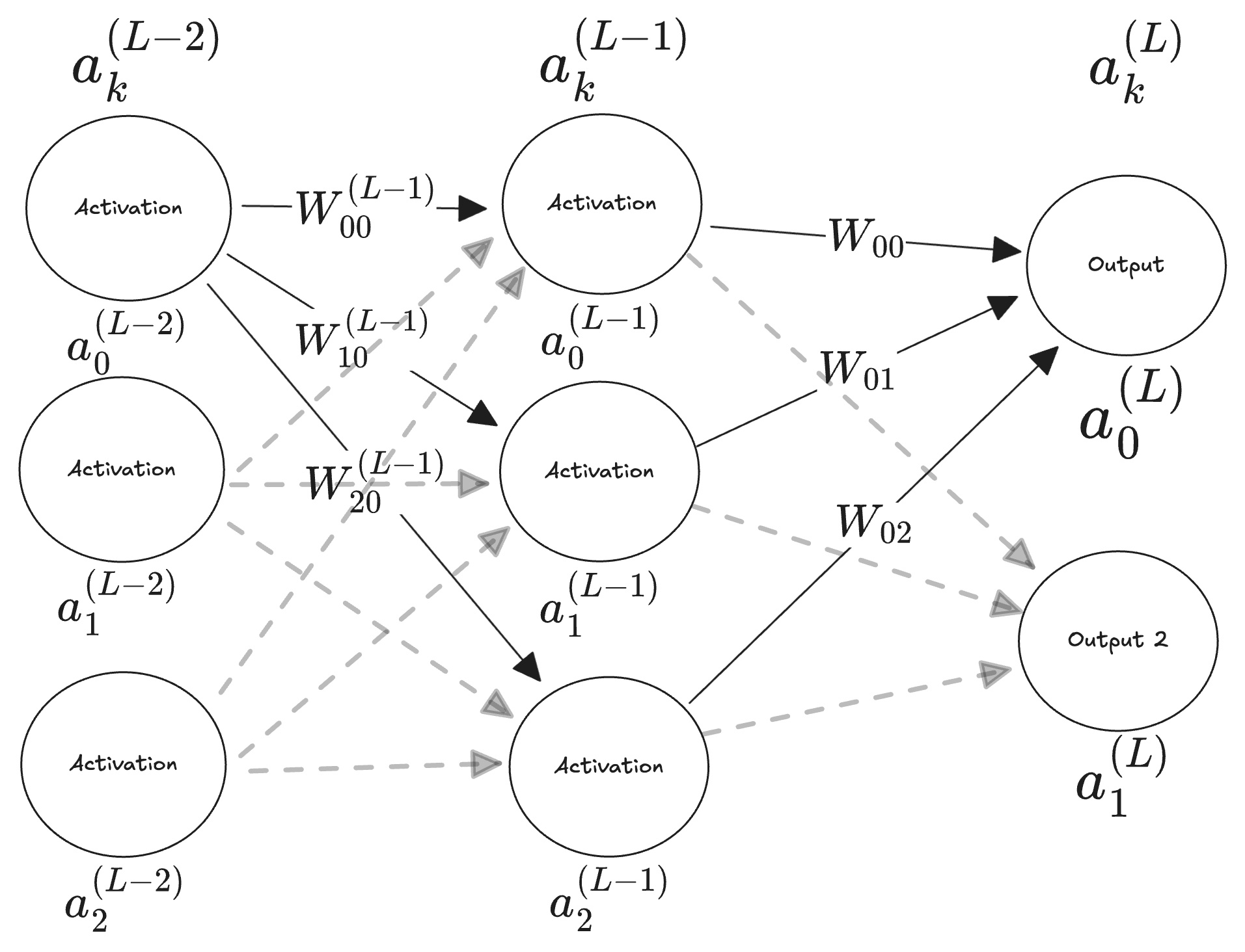
Figure 1 - Multilayer, multi-unit neural network from the last post
In the last post I said the calculation for layer L would be the weights connecting the last neurons, multiplying the activation of the neurons in the origin and summing everything, or mathematically:
$$z_j^{(L)} = w_{j0}^{(L)} a_0^{(L-1)} + w_{j1}^{(L)} a_1^{(L-1)} + w_{j2}^{(L)} a_2^{(L-1)} + b_j^{(L)}$$Two times because there are two neurons in the output layer (L)
But it is a bit too tiresome to multiply every single neuron for every layer, and do everything again for every forward pass in the training, which can extend to thousands of training inputs.
So let’s rewrite using matrices:
Since layer $L$ has 2 neurons (Output, Output 2) and layer $L-1$ has 3 neurons, the weight matrix is $2 \times 3$:
$$\begin{bmatrix} a_0^{(L)} \\ a_1^{(L)} \end{bmatrix} = \sigma \left( \begin{bmatrix} W_{00} & W_{01} & W_{02} \\ W_{10} & W_{11} & W_{12} \end{bmatrix} \cdot \begin{bmatrix} a_0^{(L-1)} \\ a_1^{(L-1)} \\ a_2^{(L-1)} \end{bmatrix} + \begin{bmatrix} b_0 \\ b_1 \end{bmatrix} \right)$$Simpler, right? Now we can visualize everything in one block without getting too much information.
Reminder, matrices are represented in row and column, $M_{RowxColumn}$.
Multiplying two matrices $M_{2x3}$ and $N_{3x1}$, the output takes the rows of the first and the columns of the second, so MxN = $R_{2x1}$ (which is our case)
Summing matrices keeps the dimensions and just sums element by element.
You can also think of it like this: for each activation neuron there will be one row of weights, one column of activations from the last layer with N rows, and one column with one bias for each activation neuron.
It’s easier to process more data in one batch this way because the data is collapsed in matrices.
Basic training techniques (Batch, Small-batch and SGD)
Considering the matrix calculations, let’s jump to training techniques. By techniques I mean ways of processing the data. For example, you can update the gradient descent in the training considering one dataset input, multiple inputs or even the whole dataset for every step. Abstractly, you can think of it as running towards the minima based on each input, on the batch or on the dataset as a whole.
Dotting the i’s and crossing the t’s, the gradient descent calculated based on the complete dataset for every step is the batch training, the sliced dataset would be the mini-batch training, and the version that updates for every input is the stochastic one. So, we have the batch gradient descent, the mini-batch gradient descent and the stochastic gradient descent.
This plot is a convex surface and the lines are proceeding towards the minima:
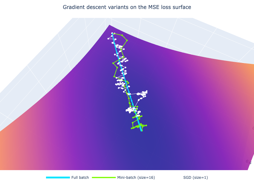
Figure 2 - Batch, mini-batch and SGD paths towards the minima
The SGD in the subtitle is white… I noticed too late, sorry. Also the gradient goes from lowest to highest as blue to orange
We can see the difference in routes but they end up at least close to each other in the end. The end here stands for the decreased error surface point.
This next plot is the comparison between the error calculation and the number of steps. The purpose of this one is to emphasize the increase in steps and the decrease in mathematical complexity for each processing step. It’s important to remember that computers are much more efficient at simpler but parallel tasks than at intensive individual tasks, even more so if we consider the GPU (graphics processing unit). As already explained in the memory post, these units are perfect for these matrix calculations, and you can parallelize thousands of executions (important to say that execution here doesn’t mean steps but smaller steps like weight updates or forward processing for example)
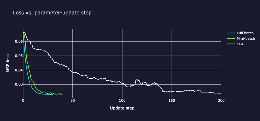
Figure 3 - Error against the number of steps for each technique
But even memory parallelization hits a ceiling. I plotted the relation between the total processing time and the MSE reduction and it gets clear that the curve which reaches the MSE minimal line faster is the mini-batch one.
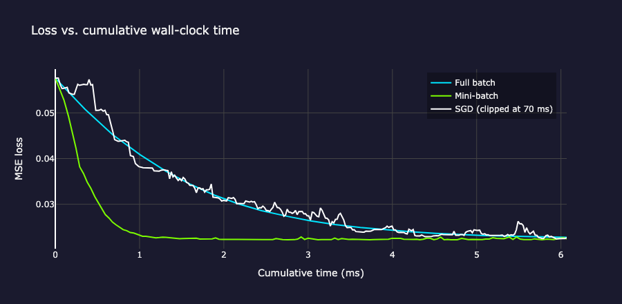
Figure 4 - Cumulative wall-clock time against MSE reduction
With that in mind, we can reach the next step, which is applying all of that to the first industry-usable tool worldwide, aka the CNN for recognizing handwriting.
Convolutional Neural Networks (CNN)
The first industry product with real evaluation using neural networks was number and letter handwriting recognition. In the US it was used to help the mail service automate zip codes and also to sort handwritten digits on paper for the financial sector. Earlier, the problem for image processing was the size and the absence of spatial context information, because everything gets flattened.
The intuition for this one is more direct. If you want to evaluate something you have to get the data from somewhere. Naturally you will select the training data to make the output more reliable, BUT if you just select anything as training, the output will also be anything.
That said, we want to find a way to train the model to recognize things from an image. To do that, Yann LeCun in 1989 published this solution link which basically IS the CNN up until 2012 (the year AlexNet was released and things took another route and also exploded into other areas, but we are going to talk about that later). In the article they introduce their setup.
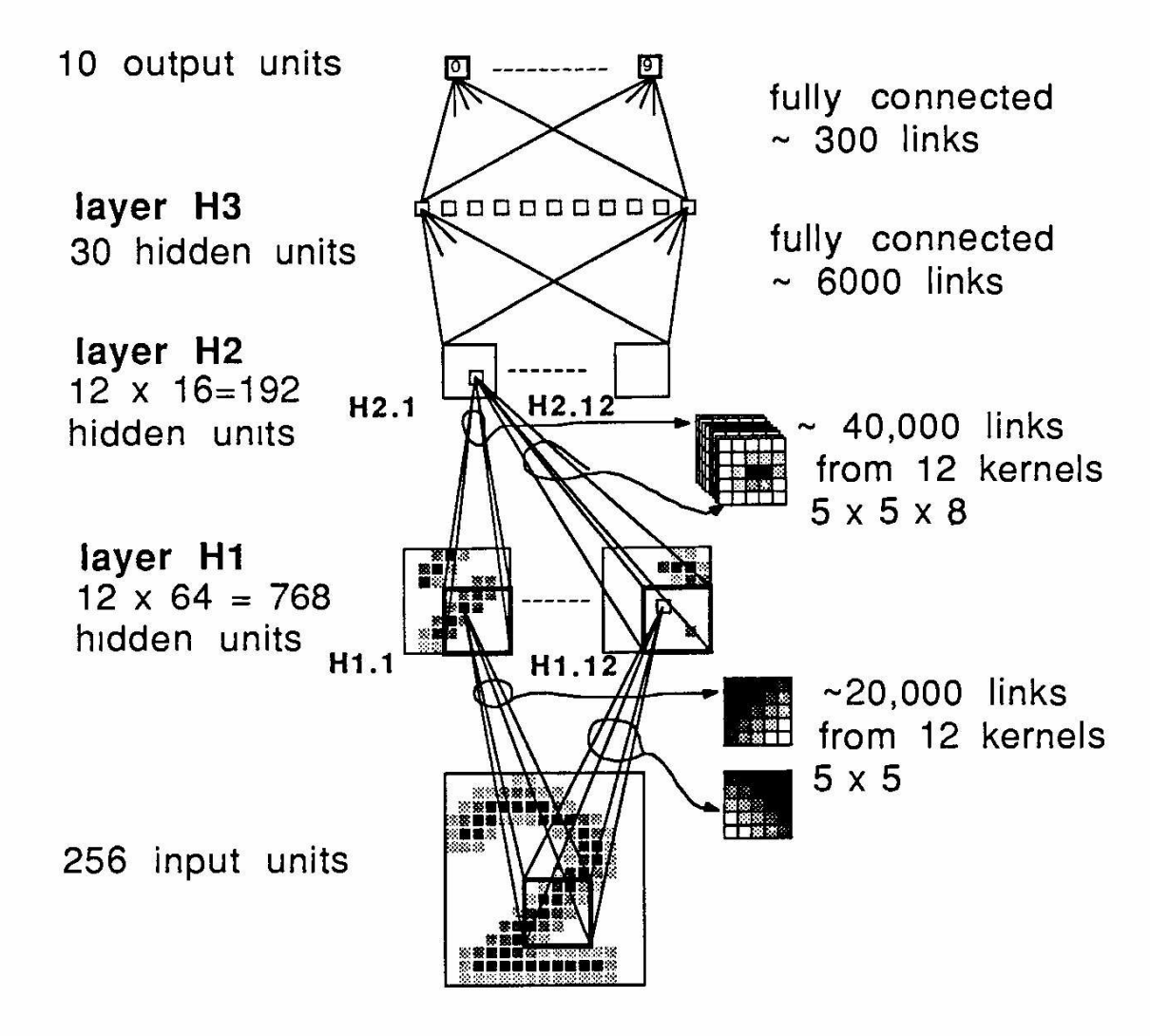
Figure 5 - LeCun’s original CNN structure from the 1989 paper
Image, Kernels and Convolution
First things first, what is a convolution? It is a mathematical operation between two functions that produces a third one, which represents how the second function influences the first one.
If you have any curiosity about convolutions, want to dive deeper, or want more intuition about what it represents in reality, I recommend the convolution video from 3Blue1Brown before the rest of this post.
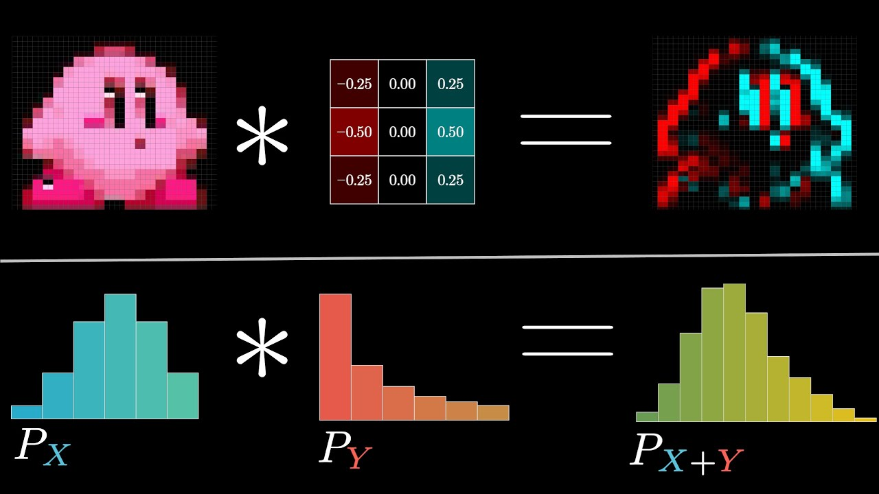
Figure 6 - Convolution example from the 3Blue1Brown video
You can imagine that the output image of Kirby represents some spectrum of the original image, like part of the original one but showing a biased type of information. That’s part of the purpose. In images, we use this kernel to make some data explicit. For example, you can blur the image to reduce its details, or run edge detection like in Kirby, which also has two color focuses based on the side, something that can be easily perceived and stands out in the output.
The function in the middle that applies the changes is called the kernel. This kernel can be seen as a weight matrix from the last post, following the first post’s idea (we’ll also need to train the weights to be more efficient at some patterns later on).
But for now let’s think about it in the same way as the perceptron, where you could manually set up some weights to distinguish a pattern that will output whether your needs are met or not. With that in mind, look at the image context. You could want to find one circle + one diagonal line and say it’s a six, but it could be a rotated nine, or it could hallucinate some other number, or even mistakenly have more than one number in the same image. We want to find a reliable way to find patterns in the whole image without any position, horizontality or verticality restriction.
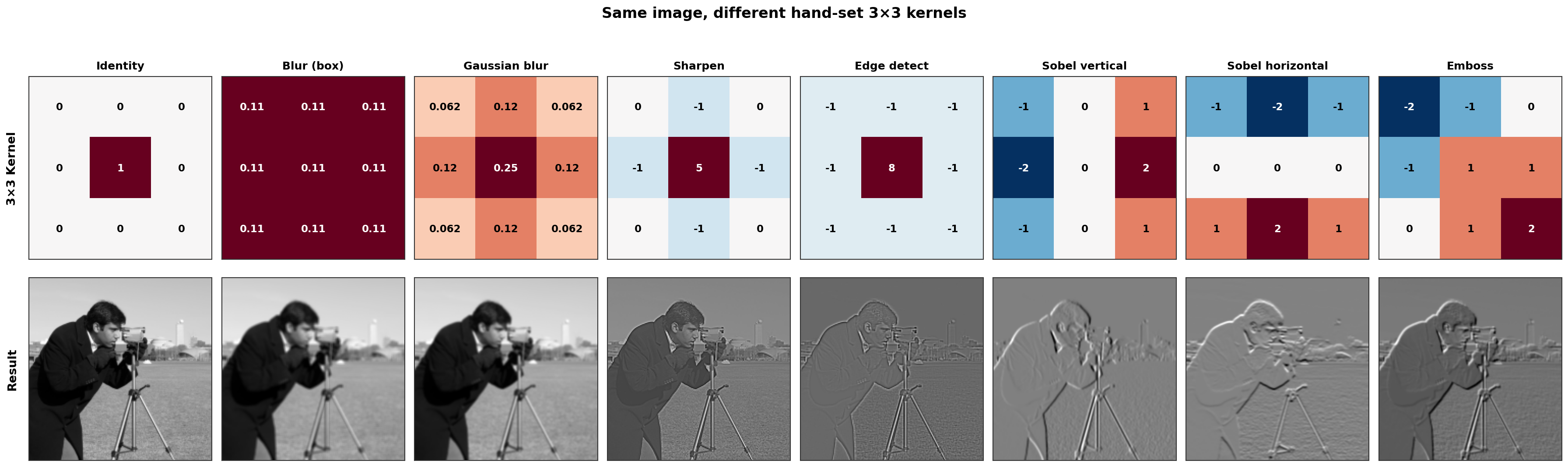
Figure 7 - Comparison of different kernels applied to an image
To do that using the LeCun technique from the paper, we run the kernel phase to make features stand out (lines, corners, shades, excess of definition and any possible thing that helps imply what is happening in the block), then run another kernel phase to make them stand out even more, and then compact all the units into a new layer with a small number of units, 30 units, and then do it again into the last layer with 10 units which represent the digits from 0-9.
Diving deeper into technical details now, observe that applying the kernel to the images will halve each spatial dimension in every one of the steps that still keeps the image format in the LeCun example. This is called Pooling. Halving each dimension drops the number of units per map to a quarter, so it goes from 256 to 64 to 16 (important to observe that the kernel “copies” still exist there but also reduced in size, and in the LeCun example there are 12 of them in all the layers after the input one). This is done intentionally to reduce the computation needed to process the later operations with weights and the backpropagation, which have to reach each one of the units in all layers.
There are some types of pooling, but to explain a bit about them I got this example of Max (the max value between the 4 units in this case) and average, which would calculate the average of the neighbouring units. (The average one blurs the image, and since every neighbour gets the same weight it is a box/mean blur)
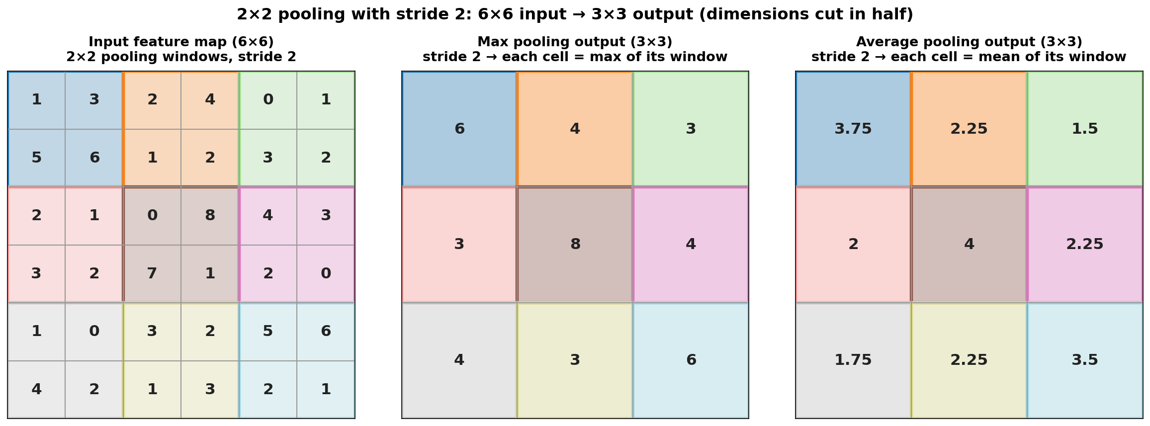
Figure 8 - Max and average pooling with stride 2
Then finally in the last layer they use a nonlinear function (remember that we need to use some sort of nonlinear function like this one, otherwise all the neurons we see are just a fancy drawing because mathematically it would collapse into one massive matrix operation), the $tanh$, to output the most “activated” weight.
In LeCun’s work they used the value range for each unit as -1 to 1 considering grayscale, in other words a black to white gradient. Because of this, the marked range in the $tanh$ is like that.
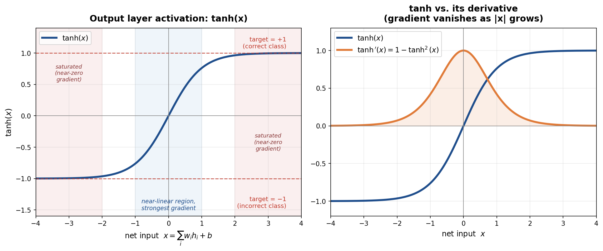
Figure 9 - Tanh activation function and its derivative
I created the second image like this to refresh the way the gradient descent works on the nonlinear/activation function, using this as a hook to say that LeCun used the mean squared error (MSE) function as the loss function. As expected, the MSE + Tanh can have some behavior that softmax wouldn’t, like two values close to the activation, but it’s okay at the end of the day because we can just get the max value itself $argmax()$, which will have a satisfying accuracy.
We already talked about that in the last post, but if you look at the derivative of the tanh, it has the biggest influence in the middle and flattens in the low and high ends. This means the biggest correction only applies when the “activation” is happening in the middle, so if a massive error value lands in it, there’s a good chance it gets stuck in the minimal correction.
We talked about that in the vanishing gradient topic but just refreshing the specific details.
LeNet-5
In 1998, LeNet-5 was released as the new state of the art for convolutional neural networks. This one improved the accuracy in overall performance and had a more structured and engineered architecture. The training dataset was almost 10x larger, now with 60,000 training images, and they used bigger images as inputs. Let’s review the changes.
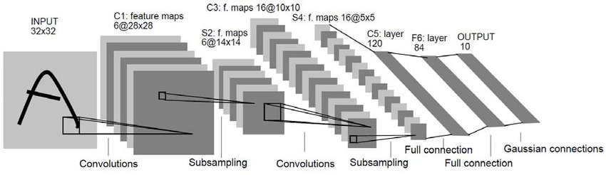
Figure 10 - LeNet-5 architecture
Now the input is twice the size, going from 16x16 to 32x32 (with padding so the edge information doesn’t get lost after the kernel process). Convolution and subsampling processes are separated (the C subtitle means convolution, S for subsampling, and F for fully connected). There are more features in the layers, one of which has 6 layers of low-level features, and the following one also has 6 layers but downsamples the previous one (keeps 6 feature maps but reduces the resolution from 28x28 to 14x14).
At convolution 3 they chose a completely different strategy from the original ‘89 CNN. The feature maps connect differently, using features from the previous sampling. Imagine this like the combination of earlier information. I said that some low-level features could be like lines, edges, etc. Now we want to combine these into newer possible information, like some “higher” level feature based on the previous one. The setup they used is:
- 6 of the C3 maps connect to 3 contiguous feature maps from S2 (maps {0,1,2}, {1,2,3}, {2,3,4}, and so on, wrapping around).
- 6 more connect to 4 contiguous feature maps from S2.
- 3 more connect to 4 non-contiguous feature maps from S2.
- The last 1 connects to all 6 S2 maps.
Now we have a new type of layer that’s based on core low-level features to improve the previous processing capacity.
Then we subsample again, reaching S4, which has a dimension of 5x5 with 16 maps. We convolve all of them into 120 independently weighted filters. This is a bit confusing, but they just used all the 16 maps with 5x5px 120x (which each time would be a different filter for the input) to produce 120 units in the layer C5. All the units generated are connected to every pixel in every map, 120 x 16 x 5 x 5, which results in 48,120 parameters. These lines connecting everything have unique weights which are gonna be trained later.
The next layer is F6, the fully connected layer, which has 84 units that can be called neurons. Till that layer we used a normal $tanh$ activation function in the training part, but it’s gonna change in the next one.
For curiosity’s sake, the 84 number is because 7x12 is the pixel bitmap used to represent stylized ASCII character images, which for now is not that important considering we just read numbers, not full ASCII, but that’s the reason for the number.
Finally, the final layer has 10 output values that represent the 0-9 range of numbers. The units don’t compute the weighted sum like normal neurons, but the distance. This one is a bit special because they changed the loss function to the Radial Basis Function (RBF).
$$y_i = \sum_{j} (x_j - w_{ij})^2$$The $x_j$ is the $j$-th value of the last layer’s 84-value vector. The $w_{ij}$ is the $j$-th value of the prototype vector, which also has 84 values.
The prototype vector is a handmade vector that basically draws the digit value in the 7x12 bitmap board so the recognizing system is guided more directly. Also, you can infer that here the system is walking towards a new breakthrough in recognizing. They are setting everything up to expand to all ASCII characters.
Since the measured value in the loss system is distance, the best output value from each sum will be the minimal one, mathematically speaking:
$$\text{predicted class} = \arg\min_i , y_i$$Training system
Considering the minimal distance system, we create a new problem, the chance of the system cheating during training, reaching some average value between all values in the prototype vector. With that, the training and everything would be meaningless.
To solve that they created a modified system for training:
$$E(W) = \frac{1}{P} \sum_{p=1}^{P} \left[ y_{D^p}\left(x^p, W\right) + \log\left( e^{-j} + \sum_i e^{-y_i\left(x^p, W\right)} \right) \right]$$$P$ is the total number of training examples, $x^p$ is the $p$-th training input, $D^p$ is the correct class label for the training input (if the image had a 6 drawn on it, the class label here would be 6).
The $y_{D^p}$ is the distance to the correct class’s prototype, given the training value and the network’s current weight $W$. So this one keeps getting smaller during training, meaning the distance keeps shrinking.
This is added to the first value inside the log, $e^{-j}$, which is a mechanism to prevent the next term from pushing values further. When the value is small enough it becomes indifferent, close to the small $e^{-j}$, so it stops getting smaller (it’s like the training incentive is designed not to run past the point where it doesn’t change anything in the system). So it just keeps the next term from making the log too small, as a margin.
And the next value in the log is what actually does the job. To make it simple, I put this plot below for intuition. The sum makes it run the operation with the $e$ for all the classes (0-9), so we get the value of $e$ elevated to the negative value of the distance between:
- Output vector from F6 for the input $x^p$
- Correct class from the prototype vector
Or simplifying, it’s the distance between the values generated from the training data and the correct vector from the prototype.
The value is negative because we want to train the log to get smaller while the distance from the class increases (to avoid the convergence to an average value I talked about before):
- If $y_i$ (distance) is small, $e^{-y_i}$ is large.
- If $y_i$ (distance) is large, $e^{-y_i}$ is close to zero.
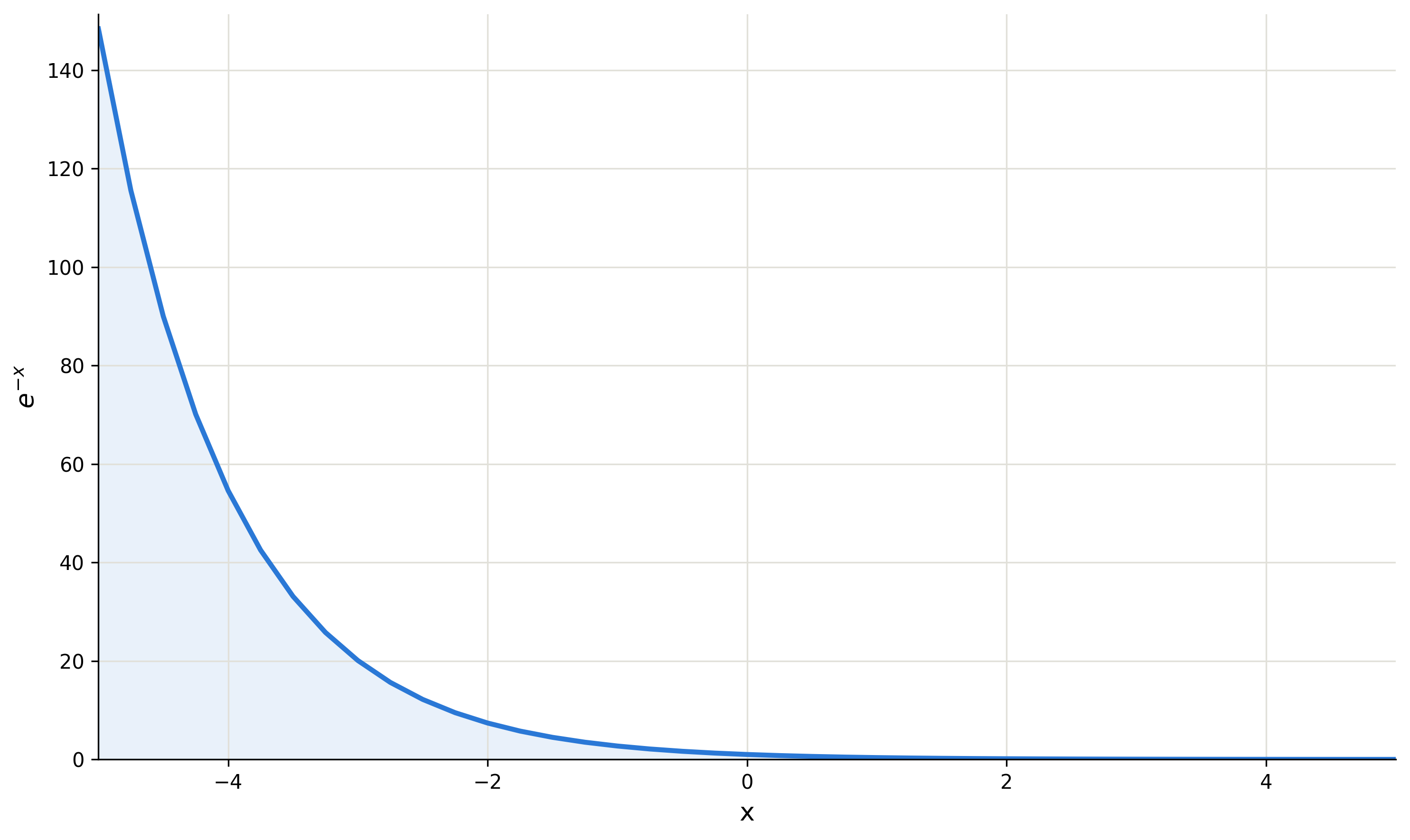
Figure 11 - e^{-y_i} decay as the distance y_i increases
Wrapping up, since the overall objective $E(W)$ is being minimized, and this term is being added, the training pushes to make this log term small too. Making $\log(\ldots)$ small means making the sum inside small, which means pushing every $e^{-y_i}$ down, which also means pushing every $y_i$ up (larger distances) across all classes.
So, this fights against the risk we talked about, the training system converging to some average value based on the prototype.
THE CATCH
Now you say, yeah, ok, but why are we getting so deep in this model’s design? LeCun’s team was good, we already got that, but this is too much, right?
No, and here I say why. This error calculation formula below also looks like a more modern formula that ended up revolutionizing the training system:
If you get the loss formula from LeNet-5 and change $z_i = -y_i$, it becomes (this change means turning the negative distance into a “score”, or, the smaller the distance, the bigger the score):
$$E(W) = -z_{D^p} + \log\left( e^{-j} + \sum_i e^{z_i} \right)$$And if you compare with the standard softmax cross-entropy loss:
$$\text{CE} = -z_{D^p} + \log\left( \sum_i e^{z_i} \right)$$It’s the same shape. The LeCun team basically reinvented the cross-entropy shape years before it became the standard for classification.
I think this is amazing.
But later on the CNN architecture dropped this fixed handmade prototype to use softmax + cross entropy mostly because of generalization possibilities with this one, which doesn’t get limited to 0-9 numbers but at some point can cover anything imaginable in images.
Training
The training also flows backwards in the same behavior as before. It also changes the weights in each connection, which in the end amounts to ~60k updates in each step:
- C1: 6 maps × (5×5 + 1 bias) = 156
- S2: 6 maps × (1 coefficient + 1 bias) = 12
- C3: 60 sparse connections × 25 weights + 16 biases = 1,516
- S4: 16 maps × (1 coefficient + 1 bias) = 32
- C5: 120 × (16×5×5 + 1 bias) = 48,120
- F6: 84 × (120 + 1 bias) = 10,164
There’s also parameter sharing going on for the layer before the kernel, not just for the kernel’s own weights. It makes sense if you think about the hardware of the time, when computation was scarce, so reusing the same few weights across every sliding position instead of having one weight per connection saves a ton of work. The backprop side of this is pretty trivial once it clicks. Since one input unit feeds into multiple output positions (and every kernel scanning it), the error sent back to that unit is just the sum of every connection it took part in, error times weight, across all of them. That translates mathematically as:
$$\sum_{k} \delta_{o_k} \cdot w_k$$And visually as:
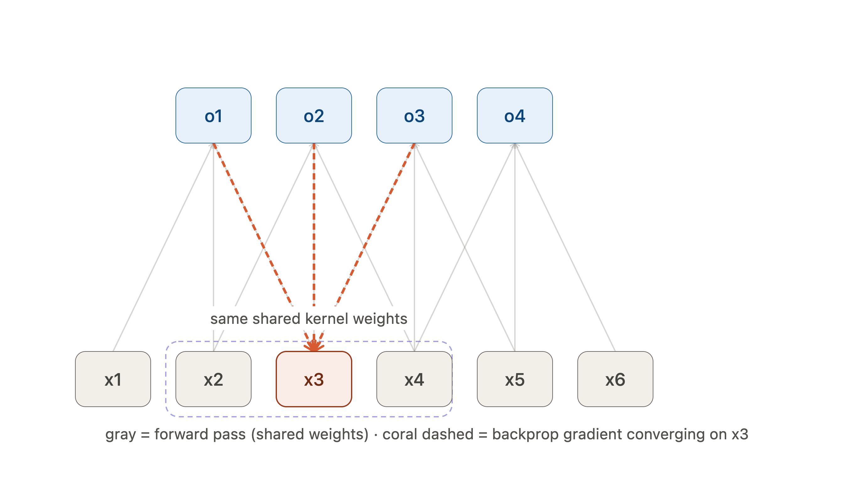
Figure 12 - Error propagation through shared weights to the layer before
Vanishing gradient
The activation used in the middle, which is $tanh$, has the same problem with any loss function, but it’s a bit worse with MSE, as I said in the last post, the gradient vanishing. The complete utilization of the value only happens in the peak of the middle graph, so usually it just uses part of the calculated value (look at the tanh vs its derivative again that makes more sense), and by calculated value I’m talking about the weight times input plus the bias that scales recursively till the last layer. So the weight updates get smaller as we go backwards.
Here Rectified Linear Unit (ReLU) comes into action for the next steps of the neural network development. It’s a simple activation function (non-linear function) that is just $f(x) = max(0,x)$, and this means that if the value is negative it becomes 0, and otherwise it keeps as is. With that, there is no shrinking in the value after the activation as happened with $tanh$, because now if the value is positive it goes forward unscathed. This also applies to backward propagation, because now the weight update doesn’t suffer from gradient vanishing anymore.
The tradeoff here is that ReLU can suffer from dead neurons, which are the ones that get stuck at 0, so there are no values to propagate forward or backwards, it becomes a dead road in the middle.
The solution is a newer Leaky ReLU, which changes the function to $f(x) = max(0.1x, x)$, which creates a possibility to recover from becoming a dead neuron, but we can talk about that later.
AI winter
After the LeNet-5 article’s release in 1998, the hype vanished for more than a decade. If you think about that, it’s basically because the theoretical field was much ahead of the practical. The training was too expensive, and the datasets available were too small for other breakthroughs. ImageNet only surfaced in 2009, which is a big dataset with images in higher quality, more labels and some diversification.
In the LeNet-5 article there were some propositions for the next steps, which could recognize more numbers in one forward pass and possibly recognize ASCII in general in the future, but at the moment were just theoretical propositions.
Also, in the last layer they used the RBF, but in the middle layers the $tanh$ kept being used. As we already talked about before, the vanishing gradient was another blocker to improving horizontal scaling (adding more layers). Another important context is that GPUs started being used for general computation later too. CUDA from NVIDIA just came to the surface in 2007, and the ML community took a couple more years to make use of that and actually build things to be used there.
With all these things happening, the funding became smaller in comparison, and therefore the number of people involved also got reduced. Add to that some alternatives that were simple and almost ready to apply in the industry, involving SVMs (Support Vector Machines), trees like AdaBoost and gradient boosting (gonna talk more about that in another post focused on statistics and calculations I guess). There were almost no reasons left to stay attached to the idea of improving the neural nets.
AlexNet
After all this lukewarm season of no breakthrough in the neural net, during the ImageNet competition in 2012 a new architecture was released and won the competition. This one is AlexNet, which got ahead of the second contender by a margin of 10.9%, which is amazing by itself considering a high-level competition like this one. They reached a 15.3% error rate in a model classifying 1,000 different categories.
The architecture they used is:
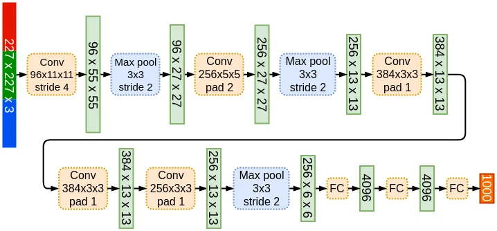
Figure 13 - AlexNet architecture Source: Packt
We can see that the basis we talked about before is still here. There are more layers, the images are denser in pixels (RGB so 3 layers for each image), and the convolutions are bigger, but that’s all there is to it. The convolution with stride I already explained before, and now it uses stride, the pace at which the kernel moves in the image, now with 3 layers.
The notation in the kernel stride: 96x11x11 means 96 kernels in each layer and 11x11 is the actual size of the kernel. About the three dimensions from the color (RGB), it gets compressed, so the kernel passes by and sums the three of them.
The max pool that appears 3 times is the type of pooling/subsampling which just gets the max value from the sampled region. Here’s an example in the image below with max and average pooling:
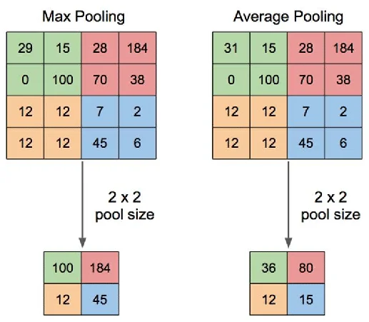
Figure 14 - Max pooling and average pooling Source: ResearchGate
For the architecture that’s all. It just increased the amount of convolution, pooling and fully connected layers. Besides that, now we have bigger images as input and the RGB feature, which opens precedent to train based on colors, too.
Training
Here it improves in many ways, but there are only a few genuinely new things considering the observations done previously in this post. They dropped the $tanh$ and started to use ReLU to solve the problem of vanishing gradient, which is one of the reasons it can be this much bigger in the number of layers. The loss function is now the real softmax + multinomial cross-entropy (also known as categorical cross-entropy loss), which is basically the shape LeNet-5’s loss already had, just without the RBF prototypes.
Binary cross-entropy (single output, two classes):
$$L = -\left[y \log(\hat{y}) + (1-y)\log(1-\hat{y})\right]$$Where $y$ is the true label (0 or 1) and $\hat{y}$ is the predicted probability (usually from the activation function).
Categorical cross-entropy (multiple classes, softmax output):
$$L = -\sum_{i=1}^{C} y_i \log(\hat{y}_i)$$Where $C$ is the number of classes, $y_i$ is 1 for the correct class and 0 for all others and $\hat{y}_i$ is the predicted probability for class $i$ from softmax. Since $y_i$ is 0 everywhere except the correct class $D$, this collapses to:
$$L = -\log(\hat{y}_D)$$Again, I recommend a video from 3blue1brown that Grant Sanderson, again, left me speechless, so here is the link. In this video he talks about cross-entropy and develops the intuition on how it works with real use cases and concrete math proofs. (He skips the Lagrange part but it’s absolutely understandable in the video).
By the way, this has the same shape as the entropy function I showed before, the RBF. But now it changed the $e^{z_i}$ to the softmax function, which comes from $\hat{y}_i = \text{softmax}(z)_i$.
The softmax function is basically a normalization function, which is gonna take all the values input $z_i$ (consider the values being the class activation) and flatten them to make the sum of all of them equal one, so if you take the max value it’s also gonna represent the activation as a percentage.
$$\text{softmax}(z_i) = \frac{e^{z_i}}{\sum_{j=1}^{C} e^{z_j}}$$The function only gets simplified this much in the loss function, because that’s the only place where the correct value is the only one class, so the other ones get canceled out by multiplying by 0. Here that’s not the case yet, it just flattens everything with the respective values being proportional to the max possible value of 1 or 100%.
Besides ReLU and cross-entropy, there are two completely new things: local response normalization (RN) and dropout.
Local response normalization
The RN is placed after the ReLU activations. Its purpose is to inhibit the neighbor neurons (vide kernels) based on the activation. For example, if one neuron activates strongly it inhibits other channels (by channels I mean the lateral block, there are multiple kernels, the output of these kernels have the same size and so on, and these are called the channels). The goal with this normalization is to make the pattern being recognized in the other channels different. If one neuron is strongly assigning something to that place, it means the other channels should look for different patterns.
This worked and improved the accuracy by 1-2%, which is really good, but later we stopped using this model for more efficient ones.
The mathematics look a bit scary but it’s simple after you understand what each variable means:
$$b_{x,y}^i = \frac{a_{x,y}^i}{\left(k + \alpha \sum_{j=\max(0, i-n/2)}^{\min(N-1, i+n/2)} \left(a_{x,y}^j\right)^2\right)^\beta}$$- $a_{x,y}^i$ is the activity of a neuron computed by kernel $i$ at spatial position $(x,y)$ (remember we are talking about images x,y is just the coordinate of the 2 dimension image)
- $b_{x,y}^i$ is the normalized output (just the result)
- $N$ is the total number of kernels (feature maps) in that layer
- $n$ is the size of the neighboring kernel window used for normalization (kernels adjacent in index, not spatially)
- $k$, $\alpha$, $\beta$ are hyperparameters
In AlexNet the parameters used were: $k=2$, $n=5$, $\alpha=10^{-4}$, $\beta=0.75$
This one works well and all, but as I said, later on we found more efficient ones, and these are Batch Normalization and Layer Normalization.
Dropout
This one is still active in basically every deep learning and neural network in general. It’s a system that during training randomly zeroes/drops part of the neurons to make it rely less on neighbour neurons. It works to keep the information concentrated in individual neurons instead of spread across a sequence, for example. It also helps prevent overfitting, which in the case of AlexNet was expected with ~60M parameters and 1.2M images.
The dropout rate is decided by testing in each architecture, but in AlexNet they used $p = 0.5$ (also only applied to the first two fully connected layers, which were FC6 and FC7). This means that in this case the chance of a neuron being dropped in each step is 50%.
Finishing
This one took more time than I expected even when I started to dedicate myself completely, so sorry for the incorrect time estimate in the video (3 days later).
Also, many thanks to my friends that keep cheering for me in continuing this process, which is so good. I love studying, and this makes it more dynamic because people drop some questions sometimes, and it’s always a pleasure to answer. See ya.
References
Papers
- LeCun et al., 1989, the original CNN paper.
- Krizhevsky, Sutskever & Hinton, 2012, the AlexNet paper.
Recommended videos